(Page 4)
Step 1 – Swept Sine Testing
The simplest test specification to analyze is that of a Swept Sine test. Figure 9 illustrates the Test Profile of a swept-sine test. The profile is an acceleration-verses-frequency spectrum, normally presented in log-log format. The acceleration amplitude is normally expressed in peak “g” units, where 1g =9.807 m/s2 = 386.4 inch/sec2. The frequency, f, is normally expressed in Hz (Hertz meaning cycle/second), though circular frequency, ω, in radian/second (1/s) is sometimes used. (Note ω=2π f = 6.2832 f.)
The test profile is (normally) composed of a series of straight-line segments. Note the frequency, f, and acceleration, g, of each point defining the end of a line segment. Calculate the corresponding peak velocity and peak-to-peak displacement for each endpoint using the following equations:


Figure 9: A Swept-Sine Test Profile is a peak acceleration (normally in g’s) versus frequency spectrum.
Retain the largest result from equation 1) as the Peak Velocity. Retain the largest result from equation 2) as the PTP Displacement. These actions are summarized for the Test Profile of Figure 9 in the following table:

Step 1 – Random Testing
Random testing involves generating and controlling a random signal with a specifically shaped spectrum and Gaussian amplitude statistics. The signal is defined by a spectral test profile called a Power Spectral Density (PSD) which is always measured and it exhibits an amplitude histogram or Probability Distribution Function (PDF) which can also be measured. Figure 10 illustrates these two complimentary views of a random acceleration.
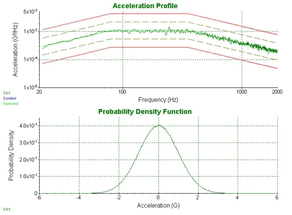
Figure 10: Two views of a random acceleration – PSD upper, PDF lower.
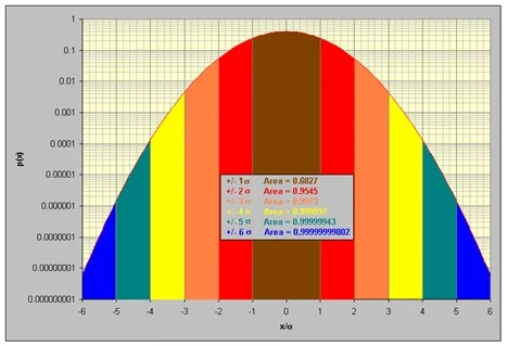
Figure 11: Two views of a random acceleration – PSD upper, PDF lower.
Like a swept-sine test, a Random test has an acceleration spectrum as the Test Profile. However, the vertical units of the random spectrum are very different; they are in units of (gRMS)2/Hz conventionally abbreviated to g2/Hz. Such a “squared amplitude” spectrum is called a Power Spectral Density or PSD. The area under a PSD is the signal’s “power” or mean-square value. Hence the area under a g2/Hz acceleration is the square of the signal’s root-mean-square (RMS) value, grms. The “per Hertz” part of the g2/Hz unit label refers to the resolution Noise Bandwidth of the instrument that measured the PSD.
A modern vibration controller measures a PSD by using Fast Fourier Transform (FFT) processing. The FFT works upon sequentially gathered blocks of N successive signal amplitude samples separated equally in time by Δt seconds. It mathematically converts these into an N/2 point spectrum with spectral amplitudes measured every Δf = 1/NΔt Hertz. A “power spectrum” is produced by squaring the spectral amplitudes and ensemble averaging many squared spectra. The averaged Power Spectrum becomes a Power Spectral Density when the amplitudes are divided by the Noise Bandwidth. The noise bandwidth of such a measurement is kΔf, where k is determined by the “window” or weighting applied to each acquired block of N time samples. A typical value of k is 1.5 when the (very common) Hanning window is applied. A window functions (such as Hanning) is necessary to suppress spectral distortions resulting from the asynchronism between the acceleration signal and the analyzer.
Because the random testing signal exhibits “bell-shaped” Gaussian amplitude statistics, the peak value, gpeak, can be precisely estimated from, grms. The PDF is an amplitude histogram (counts or occurrence versus signal value) normalized to enclose a unit area. In vibration work it is frequently useful to present a PDF with its amplitude on a log scale as in Figure 11.
The horizontal (signal amplitude) axis can be scaled to multiples of σ, the standard deviation synonymous with grms when the signal is of zero mean value. Figure 11 illustrates such scaling and shows the fraction of area subtended by ±1, 2, 3, 4, 5 and 6σ amplitude bands. Since the total are under the PDF is unity, these areas represent the probability of the signal being within the ± bounds at any time. Figure 11 shows that a Gaussian acceleration signal of RMS value, grms, will have an instantaneous peak value within ±3 grms 99.73% of the time. In other words, if the random signal has an RMS value of grms, 3 grms is a very good estimate of the peak acceleration.