Sine Sweep in High Frequency Range
Abstract
A typical vibration test often requires running the test up to 2000 Hz or beyond. This is a tremendous challenge because the resonant and anti-resonant frequencies are often only a few hundred Hz. This article analyzes the obstacles to running a sine test over a high frequency range, including the dynamic characteristics of the Unit Under Test (UUT) and fixtures, the control dynamic range of the vibration controllers, and the sensor mounting locations. Several strategies and recommendations are then discussed with results.
Keywords: Vibration Control, Sine, Structural Dynamics, Resonances, Anti-Resonances, Average Control, Damping, Modal Survey, Dynamic Range, Sensor Mounting
Introduction
Executing a sine vibration control test is a common method of verifying the performance of the manufactured product under real world conditions. However, there are various challenges that could hinder a successful sine sweep test. These challenges include system structural dynamics (resonances and anti-resonances present in the system), sensor placement location, measurement dynamic range, and sensor quality and mounting method.
Structure dynamics - The resonances and anti-resonances present in the system can push the drive voltage to its limits. It is necessary to deal with these challenges in order to ensure the safety of the test components. Different control strategies can be implemented to overcome this challenge as discussed in the paper. In addition, sensor location is also an important aspect that must be considered while choosing the location for controlling and monitoring the sine sweep test. Information from a quick modal survey can help optimize the sensor location which further assists in enhancing the test setup. This information can also be used to avoid over testing or under testing the specimen.
Control dynamics - A low dynamic range of the controller not only affects the measurement but also affects the control. The high amplitude signals would be clipped, and the low amplitude signals will be close to the noise floor. This ultimately affects the precision of the output drive voltage at the resonances and anti-resonances which results in bad control of the sine sweep profile. To overcome this challenge, a high dynamic range is used and the dual ADC technology behind this is discussed in the upcoming sections.
Sensor quality and mounting methods - The sensitivity of the sensor and the mounting method affect the usable frequency range of the sensor. A sensor with high sensitivity would be required for a low-level vibration test to ensure a good signal-to-noise ratio. Also, the mounting method for the sensor should be taken into consideration. Care must be taken to ensure that sensitivity of the sensor does not change in the interested frequency range of operation.
To demonstrate the issues mentioned above, a sine sweep vibration control test is executed with the EDM VCS software. A sensor is mounted onto the UUT and a single shaker sine sweep test is executed in the 5-2000 Hz frequency range using a single control channel strategy. The plot below shows that the test aborts abruptly because of the system anti-resonance at 168.5 Hz.
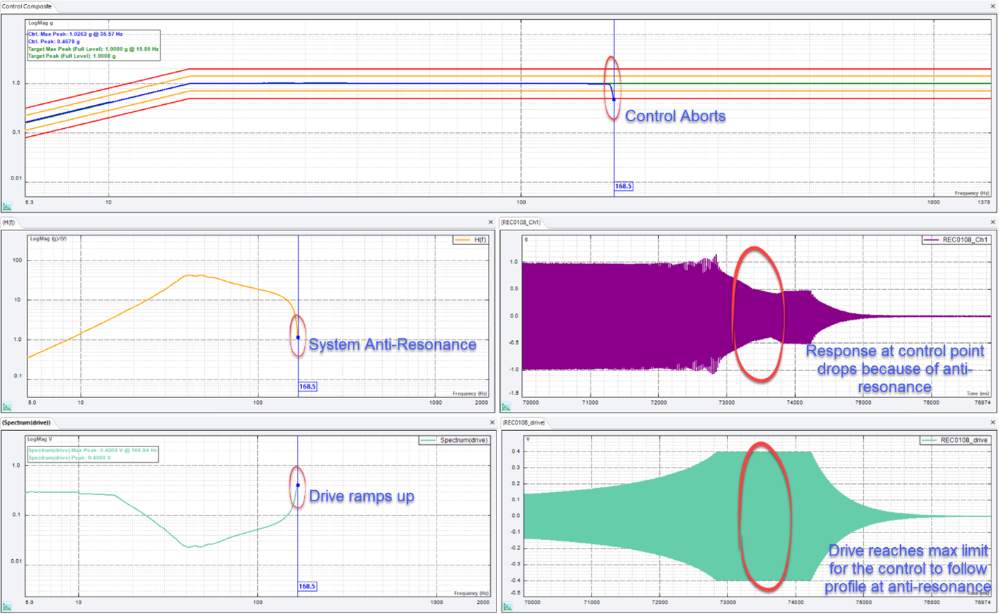
Figure 1. Issues observed in a Sine Vibration Control test
At the anti-resonance at 168.5 Hz, the drive voltage must quickly ramp up to ensure the control follows the reference profile. Even after the drive reaches the maximum limit, the response at the control location is low and continues to drop. This causes the control to drop beneath the lower abort limit, aborting the test.
This paper discusses and illustrates various strategies such as weighted average control, optimal sensor location and high controller dynamic range, all of which help achieve better control for the sine sweep test.
Outline of Sine Vibration Control Test
The digital Vibration Control System (VCS) is a computer-based system that conducts closed-loop control of vibration shaker table systems. It generates an electronic signal for a shaker amplifier that provides the drive signal to a hydraulic or electro-dynamic shaker. The vibration response on the UUT (Unit Under Test) is then fed back to the VCS controller from transducers that measure acceleration, velocity, or displacement. The controller adjusts the drive output such that the control signal conforms to specified characteristics in the time or frequency domain. There are many vibration control test types, including Swept Sine tests.

Figure 2. Hardware connection diagram for a Vibration Control test
While a Random test generates broadband signals over a band of frequencies at once, a Sine test generates one frequency, and sweeps the frequency over a defined range. Feedback from the control channel(s) is then used to adjust the drive channels’ output amplitude such that the response amplitude of the control channel(s) on the shaker table or UUT matches the pre-defined reference profile. The test profile is amplitude spectra defined as peak acceleration versus sweeping frequency.

Figure 3. Sine Control System Structure
The Sine control process consists of generating sine wave output to excite the shaker table or device under test, detecting the control signals’ input amplitudes, comparing the detected levels with the reference profiles, and updating the drive signal appropriately to achieve control.

Figure 4. Single Axis Sine Vibration Control Test in EDM VCS Sine
Usually, a sine vibration test is used to determine the performance of the UUT when subjected to the programmed profile. However, the Sine control tests sweep through the desired range one frequency at a point and hence have a much higher Signal-to-Noise ratio which produces cleaner responses. This process thus excites each of the frequencies and can be used to obtain resonances and anti-resonances for structural analysis. This information about the amplitude relationship at different frequencies can guide the user in measuring or improving the mechanical properties of the structure.

Figure 5. Basic harmonic motion equation for displacement, velocity, and acceleration
The basic equation for harmonic motion is illustrated in the diagram above. This relationship can also be used to convert the input profile values between displacement, velocity, and acceleration for the sine vibration test.
Parameters like sweep range and the sweep duration are pre-determined to test the life cycle of the specimen. Using these parameters, settings for Start and Stop frequency, time duration of sweep, sweep fashion and sweep rate, and acceleration level of the profile are programmed accordingly.
The sine sweep can be executed in a linear, log or octave fashion. To illustrate an example, a sine sweep is executed as shown below.

Figure 6. Sine sweep time signal
The reference profile for the sine sweep vibration control test consists of entering a set of input amplitudes for acceleration, velocity or displacement for the corresponding frequency points and the slope values associated with the segments. The software can automatically calculate and interchange the crossover frequency points or the amplitude values when the slope between the data points is present.
An example of an acceleration profile programmed in “g’s” vs frequency plot is shown below.
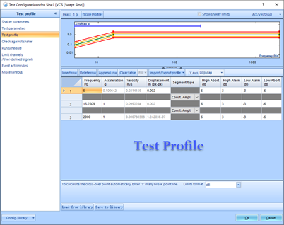
Figure 7. Example Profile for Sine Vibration Test
To ensure that the test is safely within the shaker limits, the maximum peak values of acceleration, velocity and maximum peak-peak values of displacement are displayed alongside shaker capabilities. If the programmed profile exceeds the system’s limits, the software will alert the user to adjust accordingly.

Figure 8. Shaker Limit Check
At some measurement points, the reference profile of the sine vibration test will produce some response “g” level on the UUT. The vibration experienced at the resonances would be significantly higher while the anti-resonances would experience little vibration.

Figure 9. Example illustrating input profile and output response of a sine vibration test
Challenges of Executing Sine Sweep in High Frequency Range
As briefly discussed in the prior sections, while executing a sine vibration test in a high frequency range, certain issues might appear that can affect the test operation. These may be due to the resonances and anti-resonances present in the system (head expander attached to the shaker or the test specimen), the location at which the control sensor is mounted (node of a mode), the ineffective dynamic range of the controller. These are explained in detail below with some examples to illustrate the challenges. Some strategies to help overcome these are also described.
Structure dynamics - In addition to the UUT, there are several other key components present in the system that can affect the operation range of the vibration control test. The resonances and anti-resonances of the system cause the drive to reach its low or high limit respectively which can cause a test abortion. A high drive could also end up damaging the amplifier or the shaker. Thus, it is necessary to deal with these bottlenecks to ensure a safe and efficient vibration control test. Weighted average control strategy is highly effective in overcoming this limitation. Sensor location is another aspect which needs to be considered. There might be certain locations which experience relatively lower or higher vibration than the control profile. Also, there would be certain locations where the specimen experiences little to no vibration and these are bad location points for controlling the test because the drive would exceed the limits to achieve some response at these locations. A modal survey and damping treatment helps optimize these locations for an effective test.
Control dynamics - An ineffective controller dynamic range hurts the measurement accuracy by clipping the high amplitude signals and burying the low amplitude signals under the noise floor. This in turn affects the precision of the drive that needs to be output, especially at resonances and anti-resonances. The drive will reach its lowest at resonances and its highest at anti-resonances. An inaccurate drive will also result in bad control. A controller with high dynamic range helps overcome this challenge to effectively execute a sine sweep vibration control test.
Sensor quality and mounting methods - The sensor sensitivity and mounting method also determine the frequency range of operation for the vibration control test. If the sensitivity of the sensor deviates from its nominal value, it can greatly affect the control for the programmed profile. It is also important to ensure that the sensor has a high signal-to-noise ratio for the vibration level of the control test. In addition, an appropriate mounting strategy must be chosen for the sensor such that it does not affect the sensitivity in the programmed frequency range.
These issues can be effectively overcome with average control strategy, carrying out a quick modal survey to identify optimal sensor location and using a controller with a high dynamic range as discussed in detail below.
Dealing with Structure Resonances and Anti-Resonances
The most crucial limitation that could hinder executing a sine vibration test up to high frequency ranges is the structural dynamics of the system. The complete system consists of shaker armature, head expander or slip table, fixture and UUT. Any system component can have certain resonances and anti-resonances present within the frequency range of the vibration test. For context, the head expander is usually installed to increase the surface area of the shaker armature; the test specimen is then mounted onto this head expander through a fixture to execute the sine vibration test.

Figure 10. FRF and Drive relationship along with control profile for a vibration control testFigure 3: Display Preference Setup
The combined effect of these resonances and anti-resonances of the system along with the drive voltage could cause some issues with the control. This underlines the importance of choosing optimal location for mounting the accelerometers for efficient control of the vibration test.
Executing a quick modal survey of the system helps in optimizing the physical setup. The results from a modal survey can not only provide information about the frequencies of the resonances and anti-resonances, but it can also show the node locations for each of the system modes. A node is the location where a system experiences zero response for the input drive. If the control sensor is mounted on one of these node locations, the drive voltage to the shaker would exceed the limit because the system is not experiencing any response. This is undesirable and may also ultimately damage the system because of the high drives. There can also be other concerns as it exceeds the safety limits of the test. Hence, it is crucial to understand the resonances, anti-resonances, and nodes for the different modes of the whole system.

Figure 11. FRF Plot Overlaid illustrating the system resonances and anti-resonances
As the screenshot above illustrates, the resonant frequencies for the system align and overlap very consistently, a common trend. At these resonances, even a small drive voltage will generate a high response at the sensor location. Therefore, care must be taken to ensure no damage is caused to the system during the test operation.
On the other hand, the overlaid FRFs illustrate that the anti-resonant frequencies vary from one FRF to the other. This is more crucial during the vibration control test. At these anti-resonances, the system experiences minimal vibration and hence the controller sends out a signal to increase the drive voltage for the system to experience more response. Hence, it is critical to understand and locate these anti-resonances to ensure the safety of the test. For a brief review of modal testing and analysis concepts, see Appendix A.)
Vibration Control Strategy
The vibration controller provides various measurement strategies to overcome the difficulties described above. Control strategy sets whether single or multiple control channels are used. Control strategies like maximum, minimum, average control etc. can assist in obtaining perfect control at the desired locations.

Figure 12. Various control strategies available for a Sine vibration test
In a single channel control strategy, only one input channel is used as control channel. An example screenshot of a sine sweep test executed with this strategy is illustrated below.
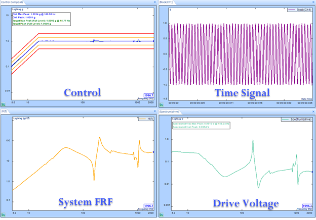
Figure 13. Sine Sweep test executed with single channel control strategy
In a weighted average control strategy, a weighting factor is applied to each input control channel and all the weighted signals are summed together to form a control composite signal. These weighted factors (wi) are defined in the input channel settings. Each control channel can have a customized weight associated to it. This allows for different weights to be assigned for each control channel. Also, equal weights can be assigned to each control channel. Following equation is used to compute the control spectrum from all individual spectrums from the sensors:

wi – weighting factor
A block diagram illustration for the control logic involved in a weighted average control strategy is shown below.

Figure 14. Control logic for weighted average control strategy
To illustrate the above example, three control sensors each assigned a weightage of 33% are used to execute a weighted average control measurement for a single axis sine sweep vibration test.

Figure 15. Sine sweep test executed with weighted average control strategy
The above plot illustrates that even though each individual control sensor experiences a drop at the three anti-resonance frequencies which is reflected in the spectrum plots, the control is perfect because it is a weighted average of the three spectrums. Also, the system FRF is different from that of the single channel test as the sharp anti-resonance is now averaged out using the data from the three control sensors. This is also reflected in the drive voltage plot, as the ramp up and ramp down for the drive is smoothened out. Thus, with weighted average control strategy, the drive voltage requirement does not have to drastically increase or decrease within a short time period to counter the anti-resonance of the structure as observed in the plot of single channel control strategy above.
The weighted average control strategy is extremely helpful when different locations of the system experience significantly different vibration levels because averaging these signals helps in optimizing the overall vibration level by tuning the drive voltage to obtain good control for the programmed profile as shown above.
Controller Dynamic Range
Dynamic range is typically derived by calculating the lowest possible amplitudes that a device can accurately measure with respect to the ability of the device to measure the highest amplitude. Using the widely accepted format for measuring dynamic range, called “Full Scale Dynamic range” (represented by dBFS), the dynamic range can be defined as:
dBFS = 20 log (VFS/VN)
VFS is the maximum measurement range of the device
VN is the system base noise
As briefly introduced before, if this dynamic range is low, then the signal measured is inaccurate and also the drive sent out by the controller is not precise and this would ultimately result in bad control of the sine sweep profile. This is extremely crucial in overcoming the structural dynamics of the system.

Figure 16. Dynamic range in a controller
At resonances, the UUT would experience high amplitudes and if these signals are clipped, an inaccurate drive would be sent out which would result in bad control. Similarly, at anti-resonances, the UUT would experience very little vibration and if these low amplitude signals are very close to the noise floor, then the precision of the output drive voltage would be bad, and this would result in control not following the programmed sine sweep profile. Hence, a controller with a large dynamic range is extremely helpful.
The patented dual ADC (Analog-to-Digital Converter) technology by Crystal Instruments is suited to acquire data accurately and at high precision when input signals have wide dynamic range. The controller automatically adjusts for signal gain without any manual operation. The front-end input channels can measure a few micro-volts up to 10 Volts with 160 dB dynamic range. The high-quality components used in the hardware ensure extremely low noise.
The two ADCs operate at different input ranges – high range and low range. The low amplitude data can be precisely captured using the low range ADC simultaneously while the high amplitude data is being captured by the high range ADC. Thus, without having the users to switch the input range, low range data can be acquired with great precision while the high range data is also being acquired simultaneously.
Combining both ADCs for the high and low range signal processing, the input channel from Crystal Instruments’ Spider hardware has the unsurpassable dynamic range of 160 dB. This would benefit the measuring and controlling of its applications.

Figure 17. Dual ADC Technology by Crystal Instruments
The dual ADCs work in parallel to measure low amplitude variations within a high amplitude input signal with great amplitude resolution and accuracy. The analog to digital conversion is executed simultaneously in the two 24-bit ADCs. The signals are passed on to the DSP for real-time processing to produce a precise match in gain, offset and phase which ensures the accuracy of the time and frequency domain signals. The dual ADCs operate at 100 mV and 10 V range each with 24-bit depth. The equivalent range of voltage measurements is close to the order of 108, which is above a 160 dB dynamic range. With the appropriate sensitivity of the sensor, the entire desired range of peak amplitudes can be measured without the need for the user to configure the gain settings. Configuration options to select the range of the input channels as either fixed at 10 V or 100 mV are also available if customization of amplitude ranges is required.
Using this technology of parallel ADCs along with the channel summation technique, the low responses (that is, anti-resonances) and high responses (that is, resonances) can be effectively measured with lower noise and without any clipping.
The pre-conditioned input signal fed through a series of amplifiers is then fed through an Analog anti-aliasing filter to the sigma-delta ADCs. The Sigma-Delta ADC which has a pass band ripple of less than ±0.005 dB. Sigma-delta ADCs sample at the MHz rate and then down sample by 256 stages making them efficient in filtering out the frequency components that cause aliasing. This further ensures that the data in the desired frequency range is accurately depicted without any attenuation by the filters or without any distortion due to aliasing.
To measure the level in the incoming control signal, the detector can use different estimators including tracking filter, or can measure the RMS, peak, or mean value of the signal. When using a tracking filter, amplitude and phase data are produced while the other measurement methods only produce amplitude data.
Tracking filters greatly reduce the noise and harmonic signals above and below the sine drive frequency. Their center frequency is always tuned to the current drive frequency, allowing all other signals to be rejected from measurement and control. The filter bandwidth can be either fixed or proportional to the current frequency.
Figure 18. Tracking Filter and Center Frequency
The Spider system continually updates the tracking filter coefficients based on the current center frequency and bandwidth. It has a stop band rejection of about –60 dB. The output of the filter is averaged to produce a control amplitude value, which is then used by the comparator to correct the output drive amplitude.
The bandwidth of the filter also affects the speed of response time of a control system. The system response time is inversely proportional to the filter bandwidth. Therefore, choosing the right bandwidth of the tracking filters is usually a trial process.

Figure 19. Sine Control Theory
The output channel of the controller is equipped with a 24-bit DAC (Digital-to-Analog Converter). Based on the range of the output voltage, the appropriate range of the DAC will be chosen to send out the drive to the amplifier. If the output voltage range is low, a lower voltage range is used such that the output can be sent with a greater precision. This would be the case at resonances. Similarly, at anti-resonances, a high output drive voltage would be sent out to quickly ramp-up and ensure the control follows the programmed profile even if the response at the frequency is low.
Sensor Quality and Mounting Methods
As briefly highlighted in the prior sections, the sensor sensitivity and mounting method also determine the frequency range of operation for the vibration control test. If the sensitivity of the sensor deviates from its nominal value, it can greatly affect the control for the programmed profile. The accelerometers for controlling and monitoring the vibration test can be attached to the desired locations in various ways. Each mounting method would have its advantages and disadvantages. Various factors like sensor location, sensitivity, accessibility, ambient conditions should be considered while choosing the best fit for the application.

Figure 20. Effect of different mounting conditions on operating range of sensor
Some of the commonly implemented methods are stud mounting, adhesive mounting, and magnetic mounting. The mounting methods affect the frequency and amplitude range of the accelerometer as illustrated above. It can be observed that a hand probe has the lowest usable frequency range though it might be a simpler setup than the other sensor mounting methods. Within a 2000 Hz range, the sensitivity deviates about +10 dB before the roll-off. Similarly, while a stud mount might be a relatively more complex setup than the other mounting strategies as it is important to account for the dimensions and locations of the holes, it has the largest operating frequency range before the sensitivity of this mounting strategy has a +40 dB deviation and rolls-off.
The adhesive mount is the most commonly used approach when using accelerometers to control a vibration test. This mounting strategy provides a long frequency range of operation before the sensor deviates from its nominal value. It is also important to ensure that the sensor has a high signal-to-noise ratio for the vibration level of the control test. If the sine sweep profile is low “g” test, then a sensor with much higher sensitivity would be required such that the measured signals are well above the noise floor. If the sensor sensitivity is low, these measurement signals would be lost in the noise floor and thus a poor signal-to-noise ratio would ultimately affect the measurement and control for the sine vibration test. Hence, care must be taken while deciding the sensitivity and the operating range according to the implemented mounting strategy for executing the sine sweep for the programmed profile of the vibration test.
Setting up and Running a Sine Sweep Vibration Control Test
Understanding the limitations discussed above and using the various suggestions reviewed can help in optimizing and efficiently executing a high frequency sine vibration test. The upcoming sections discuss the different settings and parameters that should be considered and configured on the hardware and software side of the setup for a vibration control test.
Workflow of Setting up a Sine Test
The workflow for a Sine vibration test is briefly discussed below.
Choosing the appropriate shaker that would be suitable for executing the Sine vibration test for the UUT.
Choosing an appropriate head expander to ensure proper fixturing of the UUT to the shaker armature.
Ensuring that the accelerometers are mounted firmly onto the desired locations.
To complete the physical setup, connections between the controller, amplifier, shaker, and accelerometer are established.
On the software side, the input channel settings and other test related settings are accordingly configured so that the programmed profile for the Sine vibration test can be run in the desired frequency range.
System Characterization
It is critical to characterize the system for a successful sine vibration test. For example, it is important to understand the dynamics of the head expander before mounting the UUT and executing the sine vibration test because this helps to optimize the test setup by understanding the frequency range limitation. This would also have an effect on the drive voltage required to run the test as discussed in this article.
Optimizing the Test Setup
The shaker by itself could be rated for high frequency range but it is probable that when the intermediate components like head expanders or slip tables are involved, the usable frequency range of the system will creep down. Hence, it is important to separate out the appropriate physical components to run the test in the desired frequency range. Tuning the test setup to ensure that the resonances of the system components are not present in the operating range helps optimize the test setup.
Test Fixture
Care must be taken to ensure proper fixturing of all components during the sine test. Any loose components or improper mounting could eventually end up damaging the UUT. Some details that must be addressed during the fixture design of the vibration test as listed below:
Shaker table design and hole pattern for attachment
Location and dimensions of holes, bolts, and threads for UUT mounting
UUT size, dimension, and configuration along with mounting information
Mechanical properties of the UUT
Structural characteristics of the test setup and its components
Load capacity of the head expander or slip table along with test axis information
Possible resonances of the intermediate physical components involved in the system
Vibration Test Setup Orientation
A sine vibration test can be executed with the Electrodynamic shaker or a Hydraulic shaker present in the vertical orientation or horizontal orientation with each configuration having its associated advantages and limitations.
Figure 21. Vertical configuration for a sine vibration test

Figure 22. Horizontal configuration for a sine vibration test
Shaker Setup
Choosing a suitable shaker according to the payload size and mass along with the necessary force, acceleration and displacement requirements is an important part of the vibration control test. After carefully examining the details of the physical setup as briefly highlighted above, the shaker parameters can be appropriately configured. These details are used to calculate the shaker limits to ensure the safety of the test as discussed.

Figure 23. Setup of shaker parameters and shaker limits
Sensor Location and Ensuring Test Safety with Limits
Detailed discussion in prior sections underlines the importance of choosing optimal location for mounting the accelerometers for efficient control of sine vibration test. The test setup components namely head expander or slip table, UUT, shaker armature might have some structural dynamics that might affect the operating frequency range of the test. The drive voltage requirements at resonances and anti-resonances would accordingly be affected. To overcome these difficulties, weighted average control along with enhanced dynamic range of the vibration controller can be used.

Figure 24. Structural dynamics of the system
Also, features like alarm, abort and notching along with other safety limit checks can be set up to ensure a secure and efficient sine vibration test of the UUT.

Figure 25. Different limit features for test safety
Control Sensor Strategies and Input Channel Configuration
The prior sections highlight the importance of control sensor location because the UUT may experience different vibration responses across locations. If the sensor is placed at a node (of one of the modes), then it may experience minimal to zero response. Over the whole frequency range, each sensor placed on its location would experience high amplitudes for the resonance frequencies, while very low amplitudes for the anti-resonance frequencies. This would make one control location selection to be very hard so as to achieve great control.
To solve the above issue, multi-channel control strategies available can help in working through these difficulties to execute an efficient vibration control test.

Figure 26. Control Strategies for Vibration Control
Once the sensor locations and control strategy are decided, the input channel settings for the sensors (control and monitor) can be set up.

Figure 27. Input Channel setting for a Sine Vibration Test
Test Entry
The final stage of the vibration test after setting up the shaker, mounting the test specimen, attaching the sensor, programming the sine vibration profile, and configuring the according settings for the various parameters and safety limits, is inputting the test entry for the sine sweeps.
Details about the start and end frequency, sweep direction and sweep speed, number of sweeps in plugged into the software to setup the test entry for the programmed sine vibration profile.

Figure 28. Test entry for sine vibration test
Successful Test
Using the various strategies discussed above and configuring and setting up the test according to the details discussed helps in executing a perfect sine sweep vibration test for the system in a wide frequency range of 2 kHz.

Figure 29. Sine sweep test up to 2000 Hz
Conclusion
To summarize, this paper talks about the issues that commonly appear when a sine sweep vibration test is executed in a wide frequency range. The major limitations of the structural dynamics of the system components consisting of head expander or slip table, shaker armature and test specimen is discussed. The resonances and anti-resonances of the system as a whole is illustrated and the effect of it on the drive voltage requirement is explained. The effective strategy of weighted average control is used to overcome these challenges. Furthermore, a modal overview highlights the importance of choosing optimal sensor locations for executing a good vibration control test. Another major bottleneck is explained where an ineffective dynamic range of the controller could result in a bad control of the vibration test. The details about this problem where the high amplitude signals are clipped, and the low amplitude signals are lost in the noise floor is explained and also the effect of this issue on the measurement and control for the sine sweep vibration test is discussed. The information of dual ADC technology implemented in the Crystal Instruments’ controller is presented and its accuracy and precision in effectively executing a sine vibration test is discussed. The importance of sensor sensitivity and operating range is discussed in the sensor mounting strategies. Finally, the details about the hardware arrangement and software setup is discussed to demonstrate the workflow of a single axis sine sweep vibration control test.
References and Appendix
References
[1] Spider Vibration Control (Crystal Instruments)
[2] The Fundamentals of Modal Testing (Agilent Technologies)
Appendix A - Modal Overview
This section briefly discusses about the basics of modal analysis and how the extracted modal paratmeters can be used to improve the basic test setup for a vibration control test. The FRF can be expressed in different forms as shown below. The most commonly used form is the accelerance form, which is a ratio of the acceleration to the force. If a velocity sensor is used, then a mobility form of the FRF can be obtained, which is a ratio of the velocity to the force. Similarly, using a displacement sensor will provide the compliance form of the FRF, which is a ratio of displacement to force.


Each resonant frequency corresponds to a mode and each mode has its own modal characteristics. The Multiple Degree of Freedom (MDOF) system FRF can be dissolved into a weighted sum of Single Degree of Freedom (SDOF) system FRFs, where the effect of each mode can be analyzed and evaluated.
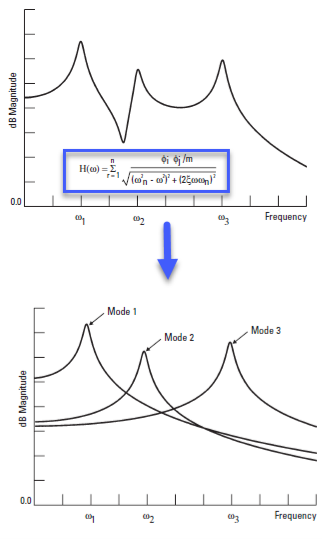
For each of the system modes, a unique mode shape along with the natural frequency and damping of the mode can be identified using the curve-fitting technique as shown above. The above picture illustrates that the FRF can be represented as a summation of the modes. That is, the FRF can be decomposed into a weighted sum of the SDOF systems as shown in the highlighted equation.
This transfer function can be expressed in various forms. If this function is expressed in terms of polynomials, properties like poles and zeros build up the transfer function. The roots of the denominator are addressed as the poles of the transfer function. The poles of the equation are the natural frequencies which provide the free vibrations of the mechanical system. Also, roots of the numerator polynomial constitute the zeros of this transfer function. Expressing this transfer function in the format shown above, the poles and residues (or mode shapes) of the equation would constitute the properties of the system as discussed below.

With the equation expressed above, the frequency and damping are calculated for each mode. This information about the poles (natural frequency - ωn and damping ratio or factor - ζ) and residue (mode shapes – ϕi ϕj) which constitute the modal parameters, is then used to understand the modal characteristics. Another observation about the peak (resonances) and valleys (anti-resonances) can be noticed. The resonances for each of the modes align and add up to produce a system resonance as illustrated by the peaks. As briefly mentioned, a weighted summation of the SDOF FRFs would produce the synthesized FRF. However, the anti-resonances or valleys could vary and may not necessarily line up or sync for each of the modes. Therefore, this modal information helps to guide the vibration control test setup because the response at these anti-resonances would be significantly low. Consequently, the drive voltage from the controller would have to be really high at these anti-resonant frequencies.
Processing the FRFs obtained from the modal survey to curve-fit them and obtain the natural frequency, damping and mode shapes provides more in-depth information about the complete system which can help in choosing optimal sensor locations.
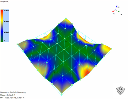
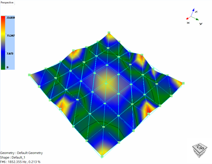
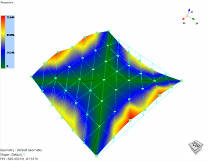
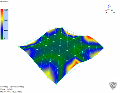
Figure 32. Mode Shapes of the head expander
The mode shapes have a contour plot displayed which shows the maximum and minimum areas of response for each of the modes. If a sensor is placed in the red or yellow region, then it experiences high response even for a small excitation. If the sensor is placed in one of the blue regions, then it experiences low response for the same input. However, the black line, also known as the node lines for each of the modes, is the place where the structure experiences no response. Care must be taken to avoid these node locations for mounting the control sensor to avoid high drive voltages.
Furthermore, this information can also be used to change the mechanical properties to shift the resonances and anti-resonances. By changing the stiffness or adding mass to the system, the resonances and anti-resonances can be pushed out of the desirable frequency range for the vibration control test. Also, performing some damping treatment on the system can help even out the structure vibration by reducing the vibration levels experienced at resonances, and increasing the vibration levels at anti-resonances. This is illustrated in the following screenshot. The sharp peaks and valleys become smoother and flatter as damping increases.

Figure 33. FRF overlay with different damping ratios