Multi-Resolution Random Vibration Control
In many vibration control testing standards, the frequency axis is drawn to a logarithmic instead of linear scale. A few typical required test profiles from Mil-STD-810G are shown in Figures 1 and 2.

Figure 1 - Figure 514.7C-9, Category 9 from MIL-STD-810G w/ Change 1 – Helicopter Vibration Profile (Sine over Random)
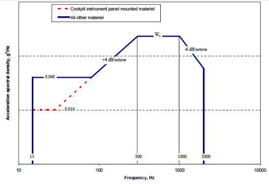
Figure 2 – Figure 514.6C-6, Category 7 – Jet Aircraft Vibration Exposure
Before we introduce the method of multi-resolution spectrum, all the vibration controllers in the market use FFT, a method which only provides linear frequency scale with uniformed resolution. In other words, what we do with the controller is not done in the current industry.
The method of multi-resolution spectrum developed by Crystal Instruments is a modification to the single pass FFT. The basic concept is that it applies two or more passes of FFT to the same incoming time streams and creates a synthesized spectrum in the frequency domain, where the frequency resolution varies. How this works with two-pass FFT is shown in Figure 3.
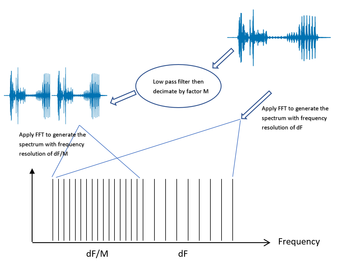
Figure 3 – Multi-resolution spectrum with two-pass FFT
The method of multi-resolution spectrum analysis can be further extended into the control process. This means that the output signal computation will come from the measurement spectrum based on multi-resolution spectra.
To increase the control performance in the low-frequency range while maintaining a reasonable loop time, different resolutions can be applied to the low and high-frequency range in the entire control process.
In the implementation of Crystal Instruments’ Random controller, two different control loops with different sampling rates are used. Suppose that the sampling rate in the control system is Fs, we divide the whole frequency range into two bands: (0, Fs/20) and (Fs/20, Fh). ΔF is the resolution in frequency band (Fs/20, Fh), then we use ΔF/8 as the resolution in (0,Fs/20]. Down sampling 8 is used in the algorithm. Figure 4 shows us the multi-resolution control method to be used.
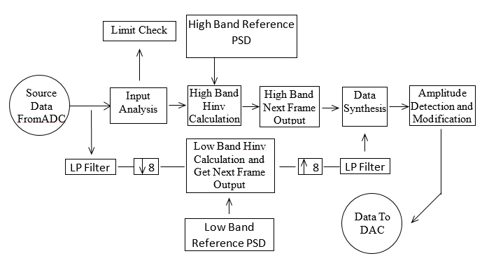
Figure 4 – Multi-resolution Control Method
The user defined profile shall be decomposed into 2 bands in the initializing period, to get the low band reference profile as shown in figure 5. The Spider controller from Crystal Instruments will operate on these two profiles simultaneously.
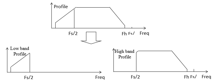
Figure 5 – User Defined Profile Decomposed into 2 Bands
In the composite windows below (Figures 6 and 7), a comparison is made between a test with and without multi-resolution spectrum control. The FFT line is set to 400. The frequency range is 2 kHz. In the plots, the green line is the target profile. The black line is the conventional control spectrum signal at frequency resolution of 5 Hz. The blue line is the one with multi-resolution turned on. The blue line has two resolutions in the whole frequency range: in high frequency band it is 5 Hz, while in low frequency band it is 0.625 Hz.
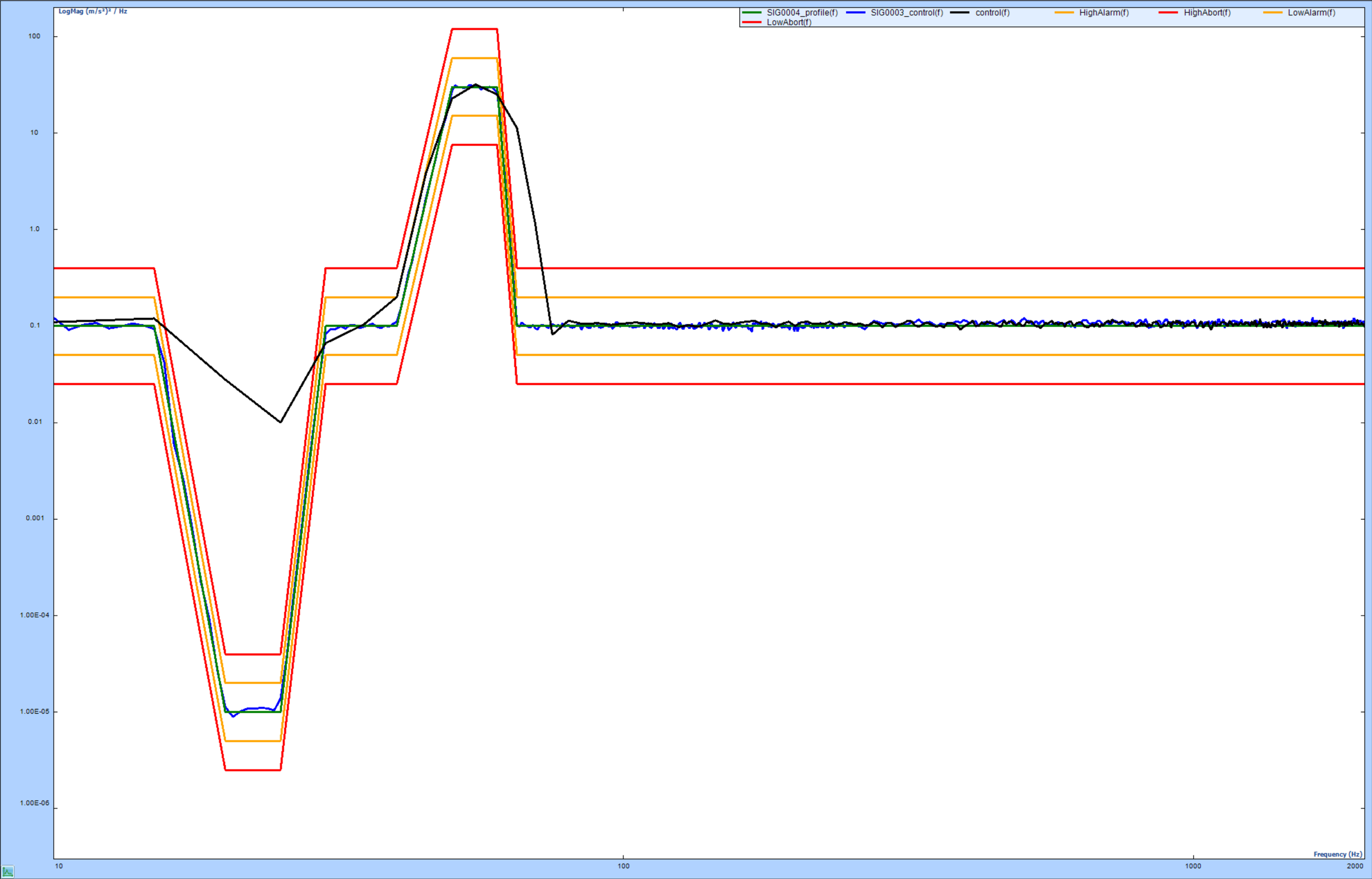
Figure 6 – Test Results Combined
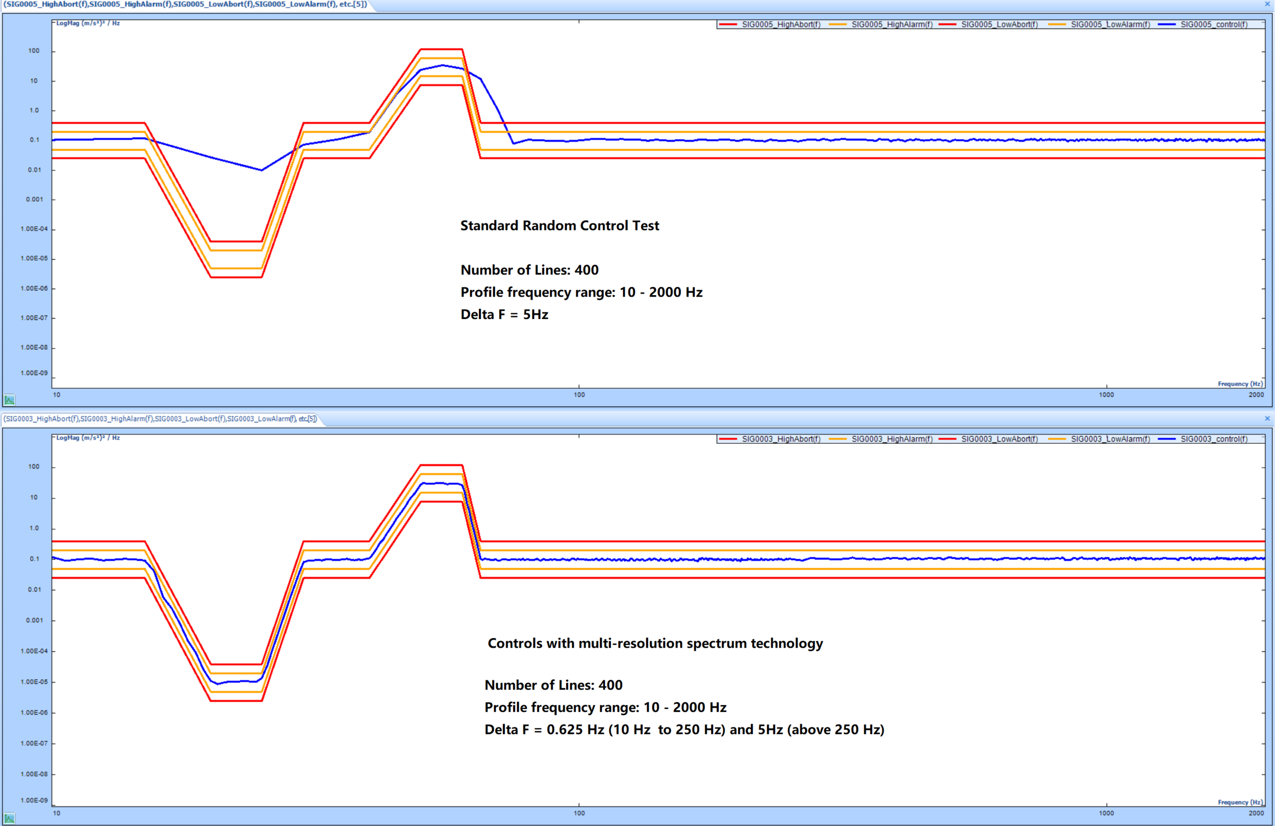
Figure 7 – Test Results Shown Separately
Obviously, test results with multi-resolution spectrum control are much better than test results without. It is common to see a 20 dB or more improvement of the control dynamic range in the low-frequency range.