PID control is a very simple and powerful method for controlling a variety of processes, including temperature.
Suppose you have a Process (e.g. a temperature chamber with heater and compressor) which produces a measurable Process Variable y (e.g. the temperature measurement in the chamber). The Process is controlled via a drive signal u that comes from the controller, and your goal is to match the PV to a target value, also known as the Setpoint, or ysp.


The acronym PID stands for "Proportional, Integral, and Derivative". Each cycle, the PID controller calculates the next output value using the measured error between the Setpoint and measured Process Variable, as shown in the above diagram. It computes the output value as the sum of the following three values:
- Proportional term: take the error and multiply it by a constant Kp
- Integral term: take the cumulative total error and multiply it by a constant Ki
- Derivative term: take the rate of change in error and multiply it by a constant Kd
Finally, it adds all three of the above values together to produce the final output u for that cycle
The above description can be aptly described in the following formula:

where:
- u(t) is the drive coming from the Controller, into the Process, at time t
- e(t) = ysp(t) - y(t) is the difference between the setpoint and measured process variable at time t
- Kp, Ki, Kd are the respective P, I, and D constants
Note: Crystal Instruments products will use a slightly different formulation for these three constants, as will be discussed below.
The performance of the PID algorithm depends heavily on whether appropriate PID parameters have been selected. If the PID constants are a good fit for the process, the control will converge smoothly. On the other hand, if the PID constants are chosen poorly, the system may oscillate or destabilize and lose control.
PID constants are ultimately determined by the user and can be refined through a combination of tuning algorithms and trial / error. Two popular methods for PID tuning are the Ziegler-Nichols and Åström-Hägglund tuning methods.
Using the Alternate PID Formulation
There are two common formulas used to describe the PID control algorithm. The first formula was already described in the above section.

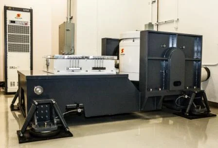
However, for the remainder of this text, we use a second framing of the PID equation:

where:
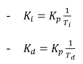
There are several reasons for using this alternate formulation:
- This allows for the constants Ti and Td to be expressed in units of time (in fact, these constants are sometimes known as the “Integral time” and “Derivative time”, respectively)
- Kp can be interpreted as the overall “gain” of the PID controller, with increases or decreases to Kp being fairly applied to the integral and derivative terms as well
- The Ziegler-Nichols and Åström-Hägglund tuning methods both use this form for their parameter recommendations
Note: the Ti (integral time) constant is in the denominator of the formula. This means that increasing Ti will decrease the integral contribution to the PID controller output, while decreasing Ti will increase the integral contribution.
Discrete Form
When digital controllers are used for PID control, the incoming data is discrete and sampled, rather than continuous. Suppose the incoming Process Variable y is sampled at intervals of T seconds:
y[k] = y(kT)
The PID formula is then converted to the following form:

- e[k] = ysp [k] - y[k]
- T is the sampling interval (i.e. the length of time between consecutive samples)
Note that the integral and derivative terms are multiplied and divided by the sampling interval T, respectively.
PID Components
To help understand each component of the PID algorithm, we will simulate each control aspect on a fake temperature chamber. This chamber is based off open-loop data from a real temperature chamber and written using Python.
Proportional Control
The simplest part of PID control is the Proportional component. Suppose you began with just a Proportional controller:
u[k] = Kp e[k] = Kp (ysp [k] - y[k])
This control adjusts the existing output in proportion to the current error measured. Below are some simulated tests with various Kp values (0.1, 0.5, 0.7):

Insights and takeaways:
- A higher Kp will help the Process Variable reach the Setpoint at a quicker pace, as shown comparing the first two plots
- Too high of a Kp will result in uncontrollable oscillations, as shown in the last plot
- Even with a balanced Kp constant, there is always some static error, which will depend on the process being controlled.
Integral Control
The purpose of introducing the Integral component is to address the static error in the process.
Static error can be explained with the example of controlling a helicopter’s elevation. Suppose you could control the height of a helicopter by controlling the rotor speed. A faster rotor speed will help the helicopter rise, while a slower (or zero) rotor speed will leave the helicopter to fall towards the ground.
If you were to only use Proportional control, then every time the helicopter reaches the Setpoint elevation, it would simply stop spinning its rotor since the error between Setpoint and Process Variable is zero! Once the rotor speed is zeroed, the helicopter would fall towards the ground, prompting the rotor to restart. In effect, the helicopter will never quite reach the Setpoint and instead hover at a slightly lower elevation below the Setpoint.
The purpose for integral control is to eliminate this static error by guaranteeing a constant component of output in the e=0 scenario, while adding the Proportional control on top. In the helicopter analogy, the integral component will settle on the perfect amount of rotor speed needed to counteract the standing effect of gravity.
The combination of Proportional and Integral control is known as PI control. Below, we show the effects of PI control in our chamber simulation:

In the above diagrams, the first plot shows Proportional control without any Integral component - as mentioned earlier, the static error cannot be eliminated.
In the second plot, Integral control is added (Ti=20), but the Integral component is too strong for the delayed temperature chamber process, resulting in oscillations.
In the third plot, Integral control is dialed back to a lower level (Ti=40), resulting in convergence upon the Setpoint.
For more insight, below is a matrix of various Proportional-Integral simulation combinations to better illustrate the effects of PI control:

Insights and takeaways:
Increasing either the Proportional or Integral component will help the Process Variable converge more quickly to the Setpoint, with the risk of oscillations if increased too much
Reminder: increasing the Integral component is done by lowering the Ti constantIncreasing the Proportional component means the error sum grows less quickly, because there is less time to accumulate error
Derivative Control
The final component of PID control is the Derivative component, which is a multiplier based on the rate of change in the error. The purpose of Derivative control is to provide a “dampening” effect that can help limit overshoot and converge more quickly upon the Setpoint. It predicts the future error and compensates the output ahead of time.
The simulations below show the dampening effects of the Derivative component. In general, adding Derivative control will reduce the amount of overshoot. However, after a certain point, increasing the Derivative no longer improves the overshoot and instead creates oscillations:

Anti-Integral Windup
One of the common pitfalls with PID control is dealing with Integral windup. Windup is the effect of accumulating too great of an error sum when the Process Variable is approaching the Setpoint from far away. It results in a significant amount of overshoot and inefficient control.
To understand why windup occurs, it is helpful to better understand the deeper mechanism of the Integral control.
The Integral component is the only part of the PID control process with long-term memory. While the Proportional and Derivative components help react to live errors, the Integral component is the only factor for improving the control quality over time.
Integral control is designed to accumulate an error sum that will offset any static error in the controlled process. That is, for every process environment, there is an “ideal” amount of Integral component that can perfectly offset this static error.
The natural goal and behavior for every PID controller is to adjust the error sum to the “ideal” value that, once combined with the Integral constant, perfectly offsets the static error.
The Necessity of Overshoot
The error sum is ultimately the sum of the gap between Process Variable and Setpoint over time. Given that the Setpoint is pre-determined, the controller can only affect the error sum by moving the Process Variable itself. If the controller moves the Process Variable past the Setpoint onto the other side, this is called “overshoot”.
Why is overshoot necessary? As long as the Process Variable is on one side of the Setpoint (greater than or less than), the error sum will either be monotonically decreasing or increasing. In almost all cases, the error sum will exceed the “ideal” error sum in one direction, which means the Process Variable must overshoot and cross over the Setpoint for the error sum to readjust in the other direction.
Thus, some overshoot in either direction is almost always inevitable. The PID variables are only here to help reduce the severity of overshoot, rather than remove it entirely. A successful PID control pattern may continue by overshooting back in the other direction, with each successive oscillation decreasing in amplitude until converging on the Setpoint.
Notably, the amount of overshoot depends not only on the PID values, but also on the initial conditions. If the Process Variable starts further away from the Setpoint, the overshoot will be greater because there is more time and runway for the accumulated sum to grow.
Consider the simulations below using the same PID parameters across runs starting at different initial conditions. Observe how the overshoot grows as we start further away from the Setpoint.

Saturation and Windup
The concept of windup is an exaggerated version of the above phenomenon where starting further from the Setpoint results in increased overshoot due to a longer accumulation period.
Consider the simulations below between a simple PID controller (left) and a PID controller with anti-windup logic (right). This time, the initial conditions for the Process Variable are placed further out to 15 degrees above the Setpoint.

The extreme overshoot from the simple PID controller (left) is a result of windup with an overgrown error sum. During the initial descent of the control, the accumulated error grows at an overly fast pace because the Process Variable is so far from the Setpoint.
Only until the Process Variable crosses the Setpoint (as marked by the gray dotted line) does the accumulated error begin correcting back towards neutral. However, due to the significant windup accumulated earlier, it takes more time to converge back to the “ideal” accumulated error value.
Integral windup can be combatted in a variety of ways. Usually, anti-windup schemes will do something related to limiting the growth of the accumulated error sum.
For instance, the PID controller depicted on the right uses a simple rule where the Integral error accumulation is disabled when the output is saturated (i.e. the output exceeds its maximum or minimum limits).
Common anti-windup measures include:
- Disabling the error sum accumulation when the controller output is saturated
- Disabling the error sum accumulation until the Process Variable is within a certain range (known as the “controllable region) of the Setpoint
- Resetting the accumulated error sum to zero (or another preset value from previous test runs) when the Process Variable first crosses the Setpoint
Tuning
The most important part of configuring the PID controller is selecting the PID constants Kp, Ti, Td. This process is known as “tuning” the PID controller.
Ziegler-Nichols
The Ziegler-Nichols tuning method is one of the most famous ways to experimentally tune a PID controller. The basic algorithm is as follows:
- Turn off the Integral and Derivative components for the controller; only use Proportional control.
- Slowly increase the gain (i.e. Kp, the Proportion constant) until the process starts to oscillate
This final gain value is known as the ultimate gain, or Ku
The period of oscillation is the ultimate period, or Tu - Use the following table to derive the PID variables
| Controller | Kp | Ti | Td |
|---|---|---|---|
| P | Ku/2 | ||
| PI | Ku/2.5 | Tu/1.25 | |
| PID | 0.6Ku | Tu/2 | Tu/8 |
| Pessen Integral Rule |
0.7Ku | 0.4Tu | 0.15Tu |
| Moderate overshoot | Ku/3 | Tu/2 | Tu/3 |
| No overshoot | Ku/5 | Tu/2 | Tu/3 |
To put this into practice, we first run simulations on our fake controller. We start with a low Kp value and steadily increase it until we see constant oscillations.

From the test runs above, the control stops converging and starts oscillating steadily somewhere around (it does not need to be too precise, as this entire process is based on heuristics.)
The measured period for the oscillations is about 80 seconds. This gives us the following:
- Ultimate gain Ku = 65
- Ultimate period Tu = 80
We can then derive PID values using the formula table and overlay the simulations:

Oddly enough, the "No Overshoot" or "Moderate Overshoot" PID variables perform more poorly than the classical Ziegler-Nichols values, at least for this simulated temperature chamber. This demonstrates how all these constants are still heuristics at best, and will may require manual adjustment afterwards.
Åström-Hägglund
The Åström-Hägglund relay tuning method is another popular method used to tune PID controllers. The basic algorithm is as follows:
- Select two opposing control output values (e.g. 100% heating vs. 100% cooling; 10% heating vs 10% cooling)
- Oscillate the Process Variable around the Setpoint by toggling between the two output values. More precisely:
Initially start with the output value that takes the Process Variable to the Setpoint
Every time the Process Variable crosses the Setpoint, switch to the other output value. - Continue until the Process Variable has reached stable oscillation about the Setpoint
- Calculate the Ultimate Gain Ku = 4d/πa, where d is the amplitude of control output oscillations, and a is the amplitude of the Process Variable oscillations
- Measure the Ultimate Period Tu as the period in the oscillations
- Use the Ziegler-Nichols formulas in the earlier section to compute the PID variables
To put this into practice, see the following simulation where we oscillate between 100% heating and cooling every time the Process Variable crosses the Setpoint.

Measurements from the simulation data indicate the amplitude of the Process Variable oscillation is approximately 3.95 degrees, giving us an Ultimate Gain of:

Meanwhile, the period of the oscillations is measured to be approximately
Tu=80
These results are similar to those derived from the Ziegler-Nichols method, at least for this particular simulation chamber. Especially for chamber tuning, the Åström-Hägglund relay tuning method is preferred over Ziegler-Nichols because it can guarantee oscillations with very few preparations needed.
Note: it is not necessary to oscillate between the two most extreme output values as in this example (between 100% heating and 100% cooling). Relay tuning can be done between any two output values, so long as the Process Variable can be driven in both directions with those two output values (e.g. 50% heating vs. 50% cooling, or 75% heating and 25% cooling.) The measured Ultimate Gain and Ultimate Period may vary slightly depending on system nonlinearity.
Applications in Crystal Instruments Software
The above PID theory principles are used in the Crystal Instruments Spider controller for temperature control.
PID Formula
In the CI software user interface, the PID constants Kp,Ti,Td are represented in the following form:

- the controller output to the chamber. Expressed as a percentage, i.e. a number between -1 and 1
- the error, calculated as the difference between measured temperature (Process Variable) and target temperature (Setpoint)
- is the PID output update interval at 2 seconds (i.e. the length of time between consecutive samples). Depending on software version, this length is usually between 0.5 and 2 seconds.
Controller Output
The controller output, u[k], is a percentage and therefore limited between the range of -1 and 1. If the calculated value exceeds that range, then it will be truncated to -1 or 1. A positive controller output means the heater is used. A negative controller output means the compressor / cooler is used.
This percentage is the usage rate for the chamber's compressor or heater over the next PID calculation period (2 seconds for heater, 14 seconds for compressor). These period lengths can be configured to the user's liking, but the compressor period is usually set to 14 seconds or longer to preserve the mechanical lifetime of the compressor.
For example, if u[k]=0.75, then the heater will be running 75% of the time for the next 2 seconds (1.5 seconds on, then 0.5 seconds off.)
If u[k]=-0.25, then the compressor will be running 25% of the time for the next period of 14 seconds (3.5 seconds on, then 10.5 seconds off). Since it is costly to turn on/off the compressor, the compressors are instead designed to use the heat bypass valve when turned "off".
PID Tuning
The PID constants are tuned using the Åström-Hägglund relay tuning method. By default, the output will oscillate between 100% heating and 100% cooling about a setpoint, but it is also possible to configure the “amplitude” of this output oscillation, such as 5% heating vs. 5% cooling.
Due to the nonlinearity in the temperature chamber, we recommended selecting an amplitude close to the practical output values used when holding at a steady temperature. For instance, in practice, the compressor at 5% usage has a stronger cooling rate than 5% of the compressor’s cooling rate at 100% usage.
Anti-integral Wind-up
The CI Spider controller uses a simple measure for preventing integral windup:
- The “controllable region” is defined as anything within ±4° C of the Setpoint. The default value of ±4° C be updated in user interface settings to the user’s preference.
- If the Process Variable is outside the controllable region, the control output will be 100% in the direction of the Setpoint. The error sum is not updated
- If the Process Variable is within the controllable region, then the full PID control is in effect with the error sum being updated.